Introduction
We are interested in comparing and visualizing the difference between using L1 norm as loss function and L2 norm as loss function for simple regression tasks.
It's equivalent to solving the following optimization problem:
$$ \alpha^+ = \arg\min_x \Vert Ax - b\Vert_1 $$
- \(A\) is the row data matrix, or the vandermande matrix in our case because we want to use polynomial regression examples. (We want the column for ones to be the last column of the vandermonde matrix)
- \(x\) is the coefficients for the regression
- \(b\) is the regression value we are trying to fit
And for L2 Norm Loss function, we have:
$$ \alpha^+ = \arg\min_x \Vert Ax - b\Vert_2^2 $$
Here is our list of topics we are gonna cover in this website
- Intro
- Solving it as Linear Programming Problem
- Non-Parametric Bootstrap
- Code
- Results
Phrasing L1 Loss as a Linear Programming Problem
$$\begin{aligned} & \min_{x} \Vert Ax - b\Vert_1 \\ & \min_{x} \left\vert \sum_{j = 1}^m a_{i, j}x_j - b_i\right\vert \quad \forall\; 1 \le i \le n \\ & \min_{t, x} \left\lbrace -t < \sum_{j = 1}^m a_{i, j}x_j - b_i < t \right\rbrace \quad \forall\; 1 \le i \le n \\ =& \min_{v, x} \left\lbrace v : -v \le Ax - b \le v \right\rbrace \end{aligned}$$
Where \(x, v\) are vectors.
This is not the optimal way, nor the professional way of doing it, I will talk more about later.
There are other ways of solving this problem, somve of the alternatives includes:
- Coordinate Descend
- Non-smooth Optimization Algorithm, eg: FISTA.
- Exploting the symmetric properties of the L1 constraint to speed up computing the KTT conditions, which then, speeds up the interior points algorithm. See an link to this in the next section for more information.
CVXOPT
For solving the system, I used a thing called: CVXOPT, available here, it uses Interior Points method, implemented in python using BLAS, which I believe it's not that bad of a solution. It's also currebtly maintained by M. Andersen and L. Vandenberghe, at UCLA.
CVXOPT provides a formulation of the L1 Loss function as a LP problem that exploits the symmetric structure of the matrix to improve the complexity of the algorithm. Which I didn't use. See here for more.
Here is the code using the CVXOPT to get the coefficients for the polynomial fit on the data with the L1 Norm Loss
import matplotlib.pyplot as plt
import numpy as np
import cvxopt as cvx
import cvxopt.modeling as cvxm
from cvxopt import solvers
solvers.options["show_progress"] = False
solvers.options["abstol"] = 1e-15
solvers.options["reltol"] = 1e-10
solvers.options["refinement"] = 10

from tqdm import tqdm

def L1RegFit(X: np.ndarray, y:np.ndarray):
    assert X.ndim == 2 and X.shape[0] == y.shape[0]
    m, n = X.shape
    A = cvx.matrix(X)
    x = cvxm.variable(n)
    b = cvx.matrix(y)
    Epsilon = cvxm.variable(m)
    Lp = cvxm.op(cvxm.sum(Epsilon))
    Lp.addconstraint(-Epsilon <= b - A*x)
    Lp.addconstraint(b-A*x <= Epsilon)
    Lp.solve()
    return (np.array(x.value)).reshape(-1)
Boostrap For Confidence Interval
Bootstrap, it's one of the way to estimate the variance of the model, when we don't know enough about the original generative process behind the data and getting new data is impossible. Non-Parametric Bootstrap to be specific.
Given training data matrix \(A\), let \(\tilde{A}\) be a list subset of matrix created by sampling rows of \(A\) with replacement, \(k\) times, which means that, it's absolutely possible, for all rows of \(\tilde{A}\) to be all the same row, but that is very unlikely when we have a lot of rows in matrix \(A\)
- \(\;B\) is the number of bootstrap we want to make.
- \(\;\mathbb{II}\) variable to keep track of the number of iterations for the for loop.
- \(\;\tilde{A}\) is a matrix whose rows are sample from the matrix A with replacment, recall that the matrix \(A\) is the vandermonde matrix of all the training pints.
- \(\;Y\) constains all the rows of data predicted by all the models from the bootstrap process.
Bootstrap Psuedocodes
Let \(\mathbb{M}\) be a set that holds trained model from the bootstrap for loop.
Let \(X\) be the Vandermond Matrix for the testing data set.
for \(\mathbb{II}\) = \(1\) to \(B\)
Make Boostrap Data \(\tilde{A}\) from matrix \(A\), resampled with replacement \(k\) times.
Make model \(\alpha\) using \(\tilde{A}\).
Add \(\alpha\) to \(\mathbb{M}\).
Let \(\hat{Y}\) be row of data predict by all the models in \(\mathbb{M}\)
For \(\mathbb{M}\), \(\alpha\) in Enumerate(\(\mathbb{M}\)):
\(\hat{Y}\)[\(\mathbb{II}\), :] := \(X\alpha\)
Let \(\hat{Y}_{\text{Lower}}\) to be a row vector of the 2.5 percenttile of all columns of matrix \(\hat{Y}_{\text{Lower}}\).
Let \(\hat{Y}_{\text{Upper}}\) to be a row vector of the 97.5 percenttile of all columns of matrix \(\hat{Y}_{\text{Upper}}\).
Code Implementation
def RegBoopStrap(
                X:np.ndarray,   # regression data
                y:np.ndarray,   # labels
                fxn:callable,   # model training function
                queries=None,   # the points to query the confident interval
                trials=None,    # number of times to make the boostrap the model
                boostrapSize:int=None,
                alpha:float=5 # confidence band interval
                ):
    """
        Performs non-parametric boopstrap for regression models
    :param X:
    :param y:
    :param fxn:
    :param queries:
    :param trials:
    :param boostrapSize:
    :return:
    """
    assert X.ndim == 2 and X.shape[0] == y.shape[0] and y.ndim == 1
    assert X.ndim == 2
    assert alpha < 50 and alpha > 0
    m, n = X.shape
    trials = X.shape[0] if trials is None else trials
    queries = X[:, 1] if queries is None else queries
    queries.sort()
    bootstrapSize = m if boostrapSize is None else boostrapSize
    assert trials > 20
    assert bootstrapSize <= m, "don't recommend bootstrap size to be larger than sample size"
    BoostrapYhat = []
    for _ in tqdm(range(trials)):
        Selection = np.random.randint(0, m, bootstrapSize)
        Coefficient = fxn(X[Selection], y[Selection])
        V = np.vander(queries, Coefficient.shape[0])
        Yhat = (V@Coefficient[:, np.newaxis]).reshape(-1)
        BoostrapYhat.append(Yhat)
    OutputMatirx = np.array(BoostrapYhat)
    ConfidenceBand = np.percentile(OutputMatirx, [alpha/2, 100 - alpha/2], axis=0)
    return ConfidenceBand
Let \(X\) be the Vandermond Matrix for the testing data set.
for \(\mathbb{II}\) = \(1\) to \(B\)
Make model \(\alpha\) using \(\tilde{A}\).
Add \(\alpha\) to \(\mathbb{M}\).
For \(\mathbb{M}\), \(\alpha\) in Enumerate(\(\mathbb{M}\)):
Let \(\hat{Y}_{\text{Upper}}\) to be a row vector of the 97.5 percenttile of all columns of matrix \(\hat{Y}_{\text{Upper}}\).
def RegBoopStrap(
X:np.ndarray, # regression data
y:np.ndarray, # labels
fxn:callable, # model training function
queries=None, # the points to query the confident interval
trials=None, # number of times to make the boostrap the model
boostrapSize:int=None,
alpha:float=5 # confidence band interval
):
"""
Performs non-parametric boopstrap for regression models
:param X:
:param y:
:param fxn:
:param queries:
:param trials:
:param boostrapSize:
:return:
"""
assert X.ndim == 2 and X.shape[0] == y.shape[0] and y.ndim == 1
assert X.ndim == 2
assert alpha < 50 and alpha > 0
m, n = X.shape
trials = X.shape[0] if trials is None else trials
queries = X[:, 1] if queries is None else queries
queries.sort()
bootstrapSize = m if boostrapSize is None else boostrapSize
assert trials > 20
assert bootstrapSize <= m, "don't recommend bootstrap size to be larger than sample size"
BoostrapYhat = []
for _ in tqdm(range(trials)):
Selection = np.random.randint(0, m, bootstrapSize)
Coefficient = fxn(X[Selection], y[Selection])
V = np.vander(queries, Coefficient.shape[0])
Yhat = (V@Coefficient[:, np.newaxis]).reshape(-1)
BoostrapYhat.append(Yhat)
OutputMatirx = np.array(BoostrapYhat)
ConfidenceBand = np.percentile(OutputMatirx, [alpha/2, 100 - alpha/2], axis=0)
return ConfidenceBand
Results
The generative model we used is \(\cos(\pi x)\), on the interval (-1, 1), with constant variance of 0.01, and 20% of the data are outliers set to be at a value of exactly -3.
Model with L1, L2 norm as loss function are trained, with 300 boopstraped models and \(k = n\) where \(n\) is the number of rows of matrix \(A\).
The degree of polynomials we use to fit the generative model is: 4
Then, a confidence 99% confidence interval are produced, with a fine grid.
This is the results
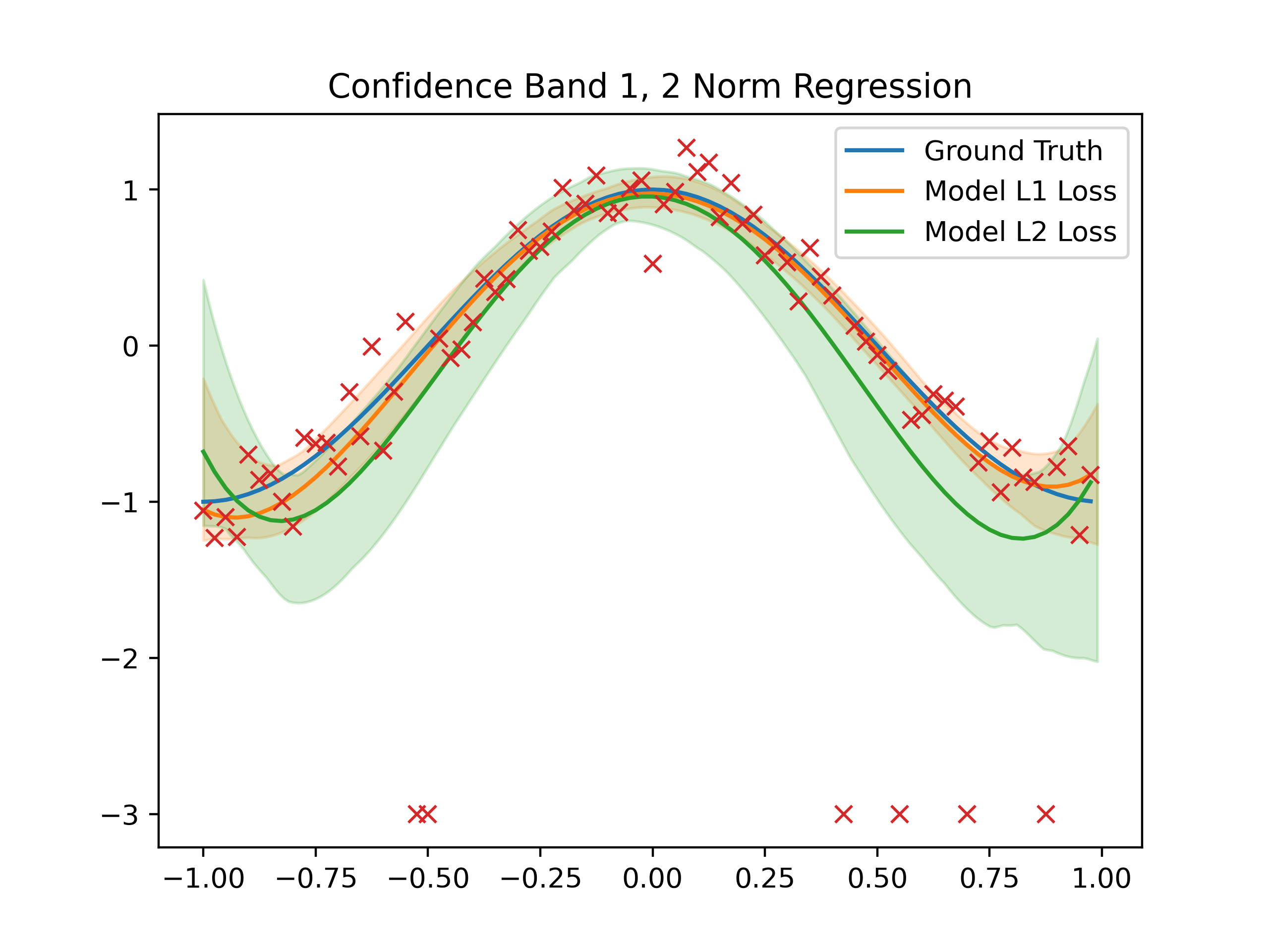
Observe that the confidence band of the model with L1 norm as loss function is narrower and its centering around the ground truth generative model. Comparing to the L2 model, which is much more suspectible to the effect of the outliers below the curve.