Introduction
The extended Knapsack problem is the Binary Knapsack problem with an additional constraints on the counts of the items allowed.
The problem can be phrased by the following linear programming problem:
\[ \max \left\lbrace \left.\sum_{i=1}^n p_i x_i \right| \left( \sum_{i=1}^n w_i x_i \right) \leq b \wedge x \leq c \wedge x \geq \mathbb{R}_+ \right\rbrace \]
Where the scalar \(b\) is the budget, the weight limit of the all the items in the knapsack and the value \(c\) is consisted of positive integers, denoting the number of a certain item that is available. The weights of the items are all real positive number and the profits of the items are real positive numbers too.
The decision value is a positive integer vector, where each element \(x_i\) denotes the number of items that are included in the knapsack.
Numerical Instability
It occurs when the algorithm is attempting to verify the feasibility of a given solution. For any given integer solution, if the purtubation on the solution vector that changes the solution from feasible to unfeasible, or vice versa.
This has a huge impact for the branching process of the algorithm. Opensource solver such as the Coint_CBC failed to address this issue, meaning that, it's also unstable. And this issue has a huge impact because it completely alters the search path of the algorithm, deviates it away from the global optimal completely.
An Instance of Instability
- Profits: [0.79, 0.35, 0.23, 0.89, 0.9]
- Weights: [0.38, 0.19, 0.01, 0.6]
- Item's count: [2, 4, 5, 4, 1]
- Budget: 1.38
Consider the following integer solution: \(x_1 = 2, x_2 = 3, x_3 = 5\). It has the following weights: \(0.38*2 + 0.19*3 + 0.01*5 = 1.38\) which saturated the total amount of available budget.
However, the python outputs the following: 1.3800000000000001, which is an infeasible solution. The binary of this number that stores in the computer memory is correct, but when converting it to an integer in base 10, it ceased to be correct. See more here.
One might doubt that: This might be an rare occurance and even if the weights are very close to the boundary, it doesn't mean that it affects the Branch and Bound process. (The following parts will surprise you if you are thinking about this), but I assure you that I didn't make up this instance by hand, It's found when via testing, and for inputs size of 5, it occurs about 1% of the time, for larger imput size, numerical instability manifested in other ways, in addition to misidentifying an infeasible solution.
The Impact on Branching
In my codes, I added a verbose mode to print out the decision made by the algorithm, and here is the outputs, let's read it together, pay attention to the pink highlighted lines of outputs from the algorithm.
BB executing with warm start solution and objective value:
{2: 5, 0: 2}
2.7300000000000004
--------------------
EKnapSack Instance:
Size: 5
Variables Aren't fixed to zero: {0, 1, 2, 3, 4}
Variable Lower Bound: {}
Greedy Soluion: {2: 5, 0: 2, 1: 2.999999999999999}
Upperbound (Objective Value from Greedy algo): 3.7800000000000002
Branching Identifier:
[?] Heuristic points to increasing objective, this node branches.
  --------------------
  EKnapSack Instance:
  Size: 5
  Variables Aren't fixed to zero: {0, 1, 2, 3, 4}
  Variable Lower Bound: {1: 3}
  Greedy Soluion: {1: 3, 2: 5, 0: 1.9999999999999993}
  Upperbound (Objective Value from Greedy algo): 3.78
  Branching Identifier: 1
  [?] Heuristic points to increasing objective, this node branches.
    --------------------
    EKnapSack Instance:
    Size: 5
    Variables Aren't fixed to zero: {0, 1, 2, 3, 4}
    Variable Lower Bound: {1: 3, 0: 2}
    Greedy Soluion: {1: 3, 0: 2, 2: 4.999999999999982}
    Upperbound (Objective Value from Greedy algo): 3.779999999999996
    Branching Identifier: 11
    [?] Heuristic points to increasing objective, this node branches.
      --------------------
      EKnapSack Instance:
      Size: 5
      Variables Aren't fixed to zero: {0, 1, 2, 3, 4}
      Variable Lower Bound: {1: 3, 0: 2, 2: 5}
      Greedy Soluion: None
      Upperbound (Objective Value from Greedy algo): -inf
      Branching Identifier: 111
      [*] Pruned by Infeasibility.
      --------------------
      EKnapSack Instance:
      Size: 5
      Variables Aren't fixed to zero: {0, 1, 2, 3, 4}
      Variable Lower Bound: {1: 3, 0: 2}
      Greedy Soluion: {1: 3.0526315789473677, 0: 2, 2: 4}
      Upperbound (Objective Value from Greedy algo): 3.568421052631579
      Branching Identifier: 110
      [?] Heuristic points to increasing objective, this node branches.
        --------------------
        EKnapSack Instance:
        Size: 5
        Variables Aren't fixed to zero: {0, 1, 2, 3, 4}
        Variable Lower Bound: {1: 4, 0: 2}
        Greedy Soluion: None
        Upperbound (Objective Value from Greedy algo): -inf
        Branching Identifier: 1101
        [*] Pruned by Infeasibility.
        --------------------
        EKnapSack Instance:
        Size: 5
        Variables Aren't fixed to zero: {0, 1, 2, 3, 4}
        Variable Lower Bound: {1: 3, 0: 2}
        Greedy Soluion: {1: 3, 0: 2, 2: 4, 3: 0.01666666666666637}
        Upperbound (Objective Value from Greedy algo): 3.564833333333333
        Branching Identifier: 1100
        [?] Heuristic points to increasing objective, this node branches.
          --------------------
          EKnapSack Instance:
          Size: 5
          Variables Aren't fixed to zero: {0, 1, 2, 3, 4}
          Variable Lower Bound: {1: 3, 0: 2, 3: 1}
          Greedy Soluion: None
          Upperbound (Objective Value from Greedy algo): -inf
          Branching Identifier: 11001
          [*] Pruned by Infeasibility.
          --------------------
          EKnapSack Instance:
          Size: 5
          Variables Aren't fixed to zero: {0, 1, 2, 4}
          Variable Lower Bound: {1: 3, 0: 2}
          Greedy Soluion: {1: 3, 0: 2, 2: 4, 4: 0.01587301587301559}
          Upperbound (Objective Value from Greedy algo): 3.564285714285714
          Branching Identifier: 11000
          [?] Heuristic points to increasing objective, this node branches.
            --------------------
            EKnapSack Instance:
            Size: 5
            Variables Aren't fixed to zero: {0, 1, 2, 4}
            Variable Lower Bound: {1: 3, 0: 2, 4: 1}
            Greedy Soluion: None
            Upperbound (Objective Value from Greedy algo): -inf
            Branching Identifier: 110001
            [*] Pruned by Infeasibility.
            --------------------
            EKnapSack Instance:
            Size: 5
            Variables Aren't fixed to zero: {0, 1, 2}
            Variable Lower Bound: {1: 3, 0: 2}
            Greedy Soluion: {1: 3, 0: 2, 2: 4}
            Upperbound (Objective Value from Greedy algo): 3.55
            Branching Identifier: 110000
            [!] This Node has found an integral solution and updated the optimal
    --------------------
    EKnapSack Instance:
    Size: 5
    Variables Aren't fixed to zero: {0, 1, 2, 3, 4}
    Variable Lower Bound: {1: 3}
    Greedy Soluion: {1: 4, 2: 5, 0: 1, 3: 0.3166666666666663}
    Upperbound (Objective Value from Greedy algo): 3.621833333333333
    Branching Identifier: 10
    [?] Heuristic points to increasing objective, this node branches.
      --------------------
      EKnapSack Instance:
      Size: 5
      Variables Aren't fixed to zero: {0, 1, 2, 3, 4}
      Variable Lower Bound: {1: 3, 3: 1}
      Greedy Soluion: {1: 3, 3: 1, 2: 5, 0: 0.4210526315789473}
      Upperbound (Objective Value from Greedy algo): 3.4226315789473682
      Branching Identifier: 101
      [~] Sub-Optimal; Branching is pruned.
      --------------------
      EKnapSack Instance:
      Size: 5
      Variables Aren't fixed to zero: {0, 1, 2, 4}
      Variable Lower Bound: {1: 3}
      Greedy Soluion: {1: 4, 2: 5, 0: 1, 4: 0.30158730158730124}
      Upperbound (Objective Value from Greedy algo): 3.611428571428571
      Branching Identifier: 100
      [?] Heuristic points to increasing objective, this node branches.
        --------------------
        EKnapSack Instance:
        Size: 5
        Variables Aren't fixed to zero: {0, 1, 2, 4}
        Variable Lower Bound: {1: 3, 4: 1}
        Greedy Soluion: {1: 3, 4: 1, 2: 5, 0: 0.342105263157894}
        Upperbound (Objective Value from Greedy algo): 3.370263157894736
        Branching Identifier: 1001
        [~] Sub-Optimal; Branching is pruned.
        --------------------
        EKnapSack Instance:
        Size: 5
        Variables Aren't fixed to zero: {0, 1, 2}
        Variable Lower Bound: {1: 3}
        Greedy Soluion: {1: 4, 2: 5, 0: 1}
        Upperbound (Objective Value from Greedy algo): 3.34
        Branching Identifier: 1000
        [~] Sub-Optimal; Branching is pruned.
  --------------------
  EKnapSack Instance:
  Size: 5
  Variables Aren't fixed to zero: {0, 1, 2, 3, 4}
  Variable Lower Bound: {}
  Greedy Soluion: {2: 5, 0: 2, 1: 2, 3: 0.31666666666666643}
  Upperbound (Objective Value from Greedy algo): 3.7118333333333338
  Branching Identifier: 0
  [?] Heuristic points to increasing objective, this node branches.
    --------------------
    EKnapSack Instance:
    Size: 5
    Variables Aren't fixed to zero: {0, 1, 2, 3, 4}
    Variable Lower Bound: {3: 1}
    Greedy Soluion: {3: 1, 2: 5, 0: 1.921052631578947}
    Upperbound (Objective Value from Greedy algo): 3.557631578947368
    Branching Identifier: 01
    [?] Heuristic points to increasing objective, this node branches.
      --------------------
      EKnapSack Instance:
      Size: 5
      Variables Aren't fixed to zero: {0, 1, 2, 3, 4}
      Variable Lower Bound: {3: 1, 0: 2}
      Greedy Soluion: {3: 1, 0: 2, 2: 2.0000000000000018}
      Upperbound (Objective Value from Greedy algo): 2.9300000000000006
      Branching Identifier: 011
      [~] Sub-Optimal; Branching is pruned.
      --------------------
      EKnapSack Instance:
      Size: 5
      Variables Aren't fixed to zero: {0, 1, 2, 3, 4}
      Variable Lower Bound: {3: 1}
      Greedy Soluion: {3: 1, 2: 5, 0: 1, 1: 1.842105263157894}
      Upperbound (Objective Value from Greedy algo): 3.474736842105263
      Branching Identifier: 010
      [~] Sub-Optimal; Branching is pruned.
    --------------------
    EKnapSack Instance:
    Size: 5
    Variables Aren't fixed to zero: {0, 1, 2, 4}
    Variable Lower Bound: {}
    Greedy Soluion: {2: 5, 0: 2, 1: 2, 4: 0.30158730158730135}
    Upperbound (Objective Value from Greedy algo): 3.701428571428572
    Branching Identifier: 00
    [?] Heuristic points to increasing objective, this node branches.
      --------------------
      EKnapSack Instance:
      Size: 5
      Variables Aren't fixed to zero: {0, 1, 2, 4}
      Variable Lower Bound: {4: 1}
      Greedy Soluion: {4: 1, 2: 5, 0: 1.8421052631578942}
      Upperbound (Objective Value from Greedy algo): 3.5052631578947366
      Branching Identifier: 001
      [~] Sub-Optimal; Branching is pruned.
      --------------------
      EKnapSack Instance:
      Size: 5
      Variables Aren't fixed to zero: {0, 1, 2}
      Variable Lower Bound: {}
      Greedy Soluion: {2: 5, 0: 2, 1: 2}
      Upperbound (Objective Value from Greedy algo): 3.4300000000000006
      Branching Identifier: 000
      [~] Sub-Optimal; Branching is pruned.
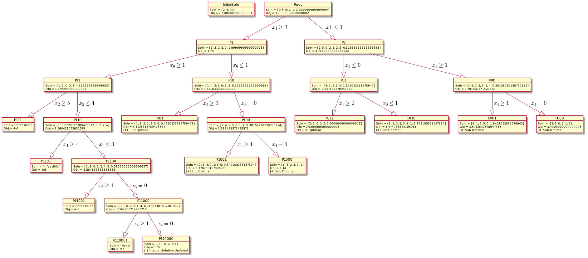
For your Covenience, I also prepare a UML diagram for illustrating the propagation of the errors:

The Graph:
- Each object is an instacne of a problem, with the greedy solution and the objective value of the solution.
- The algorithm branches from left to right in a DFS manner, that is the correct order to read the tree.
The algorithm misses the optimal solution on node: Root, P1, P11, caused another integral solution to be found at node P11000.
The error that causes the issue is not the Binary number incorrectly representing the numbers. Although, that is the true underlying problem, but the real killer behind is how the error propagage through the braching process.
Immediately after the first erronous solution caused by the binary floats representation, it propagates itself through another wave of rounding Errors. BOTH errors are affecting our algorithm.
Let's get this clear by listing them as a point:
- The rounding error, or refers to as the catastrophic cancellation error, propagates through the branch and bound algorithm because of a fixed lower bound on a certain variable.
- The representation error of binary number misidentifies the feasibility of an integer solution or vice versa, causing unwanted branching for the algorithm.
How Did I Reach the Above Conclusion
I compare the floats results with the rational computation results in debug mode. After limiting the rational computation to only the greedy algorithm part, I still failed to control the propagation of the binary representation errors. Hence, via experiments, I know the propagation of the errors on the branching process is caused by repeated summing of the floats.
Mitigating the Errors
The catastrophic cancellation error (CC Error) is a major one, the binary representation error is a minor one.
By rounding the solution, we might fix the misidentifications of feasibility of a given solution that appears to be close to an integral solution. But on the long turn, the build up on the CC Error will go back and obscure things, which in fact, causes the algorithm fails to terminate. It CYCLES around an integral solution and branches indefinitely until finally breaks off because the CC Error magnifies itself to the point of escaping the our round machanics.
However, if the CC Error is fixed then consider the case where the solution misidentified an integral solution \(x_1 = 3\) as \(x_1 = 2.999999999999999\), then immediately after, it will branch into 2 sub problems, the first is fixed on lower bound, making \(x \leq 2\) and \( x \geq 3\), and THAT! That second branch is forced to compute solution again based on the correct integral value, hence, re-crafting the solution (without the CC Error)!
In addition to the previous points, The sub-routines of the greedy algorithm that provides heuristics for the algorithm depends on the accuracy of a running sum. Or simply speaking, when the algorithm tries to figure out what is the remaining available budget of the knapsack as it adds as items decreasing in value, it's subtracting weights of the items repeatedly. And thge accuracy of that procedure depends heavily on the numerical stability.
Why Not use Rational/BigDecimals to Mitigate the Errors?
This is an important one because many programmers will be tempted to resolve the problem with provided solution in python instead of inventing their own wheels. However, here I grarantee that, this solution is absolutely not desirable.
It's not desirable for the following reasons:
- If the rational numbers are used, it has to be used for the WHOLE process of the algorithm, including the inputs and the outputs, reducing the speed significantly because rational computation is expensive.
- If big decimal is used, then a very high precision must be applied, or else, the CC Error persists when summing up big decimals repeatedly for a list of decimals.
- Using any of the above within in a limited scope on our algorithm is a waste of time because the Frary algorithm, the underlying machanics that convert the floats to rationals actually preserve the binary representation errors.
For demonstrating the third point, simply try:
import fractions.Fraction as Frac
print(float(Frac(0.57)/Frac(0.19)))
And it will still give the wrong number... And unsurprisingly, the "Decimal" in fractions does the same.
Kahan's Summation Algorithm
"Can I just use the python default sum() method?"
"ABSOLUTELY NO! NO! Please!! NO!"
"Ok ok... Jesus isn't that some over reactions there... How about the sum() in numpy"
"Yeah, that one is ok, but believe me, it's just a tiny bit better than sum() in python, and it's still way worse compare to Kahan's Summtion algorithm, because it uses pairwise Summation, a divide by conquer approach, which reduces the rate of the accumulations of CC Errors, but made no attempt to eliminate it. Another problem of that is, it doesn't support running sum in a loop."
"Finally, Python provides math.fsum function, which is as accurate as it Kahan, and I recommend using it whenever possible."
So I went ahead and implemented the algorithm for running sum, and array sum, it turns out to have a precision that is exactly the same as rational computations, very impressive, and it also provide robustness via some python special functions for data type.
This wheel is extremely simple to make, it completely eliminated the CC Error, not only that, it's easy to apply for other languages such as C++ and C# too. It's also useful for summing intensive computations, related to Matrices multiplications, getting statistical parameters, or even just improving the Nested Multiplication algorithm or polynomial evaluations.
I benchedmarked those 4 algorithms in here. And... to my surprise, the default sum() in python incorrectly summed up 95% of the floats arrays for size of 100, and np.sum() summed up 77% of them incorrectly, and Kahan's method's doesn't have any errors compare to summing up with rational numbers.
How Are These Data Computed?
I use the Numpy.sum and the sum in python to sum up floats, and I compare the results to summing up using python fractions module. The Error is the absolute value of the differences of the sums.
For each array size, I repeat the above process for 30 times and get the mean and the standard deviations. The upper bound and lower bound frame the 66% confidence interval (centered) for the true average errors. The average is ploted as the dots and the lines are the upper/lower bound of the confidence interval for each dot.
The experiment results matches the theoretical expectatsion. Numpy.sum uses pairwising summing and the error is: \(\log(N)\), where N is the size of the array. The Naive way of summing the array in the worse case, has an error that grows linear with the size of the array.
Conclusion
The nump.sum and the sum in python both has errors when summing up an array of floats, they are expetected to occur over half of the time.
The math.fsum and Kahan Summation
They both have zero errors when printed out, or more precisely: 0.0, which means that the error is on a magnitude below 1e-17. However, the math.fsum is faster and it's likely that it's optimized by python.
The Execution Time of Different Sums
I also did experiments to figure out the run-time of each of the algorithms, and here is the plot:
The Python implementation of the Kahan algorithm is not fast compare to math.fsum() in python, which shares the same accuracy.
However, the implementations for the Kahan Running sum is very easy, and it can easily be extended to support summing up sequences of comnplex numbers.
A Kahan Rumming Sum is a sum that allows the user to use the number as a accumulator, and then add floats to it in real time, making it more general and comfortable to use. It's simple and it gets the works done pretty elegantly.
The simple implementation of Kahan Rumming Sum is here.
Comparing with Pulp LP Solver
The python implementation of the algorithm has remarkable numerical accuracy, but terrible run-time compare to the Coin_CBC solver.
The initialization offset of Coin_CBC is negligible compare to the slowness of python.
But, over all the algorithm serves a great prototype for constructing the EKnapSack solver in other languages. And it demonstrated things well.
The sample size for both boxplot is the same.
Gallery
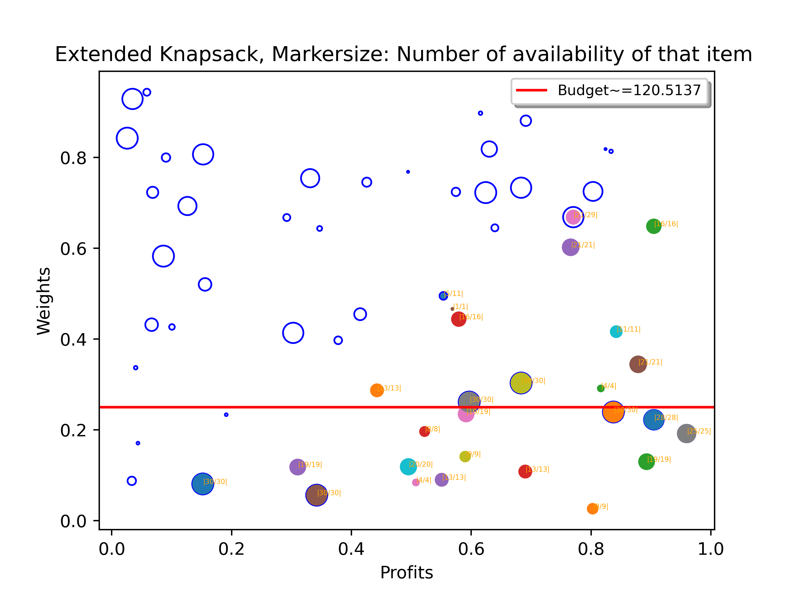
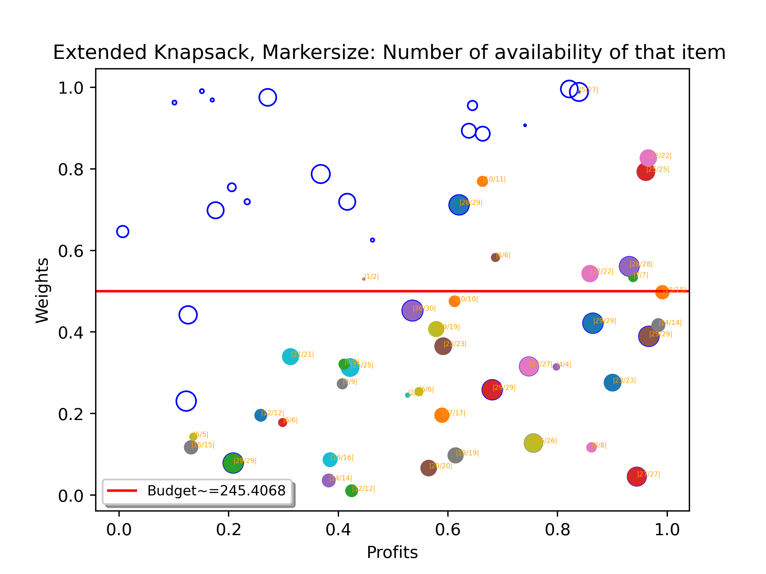
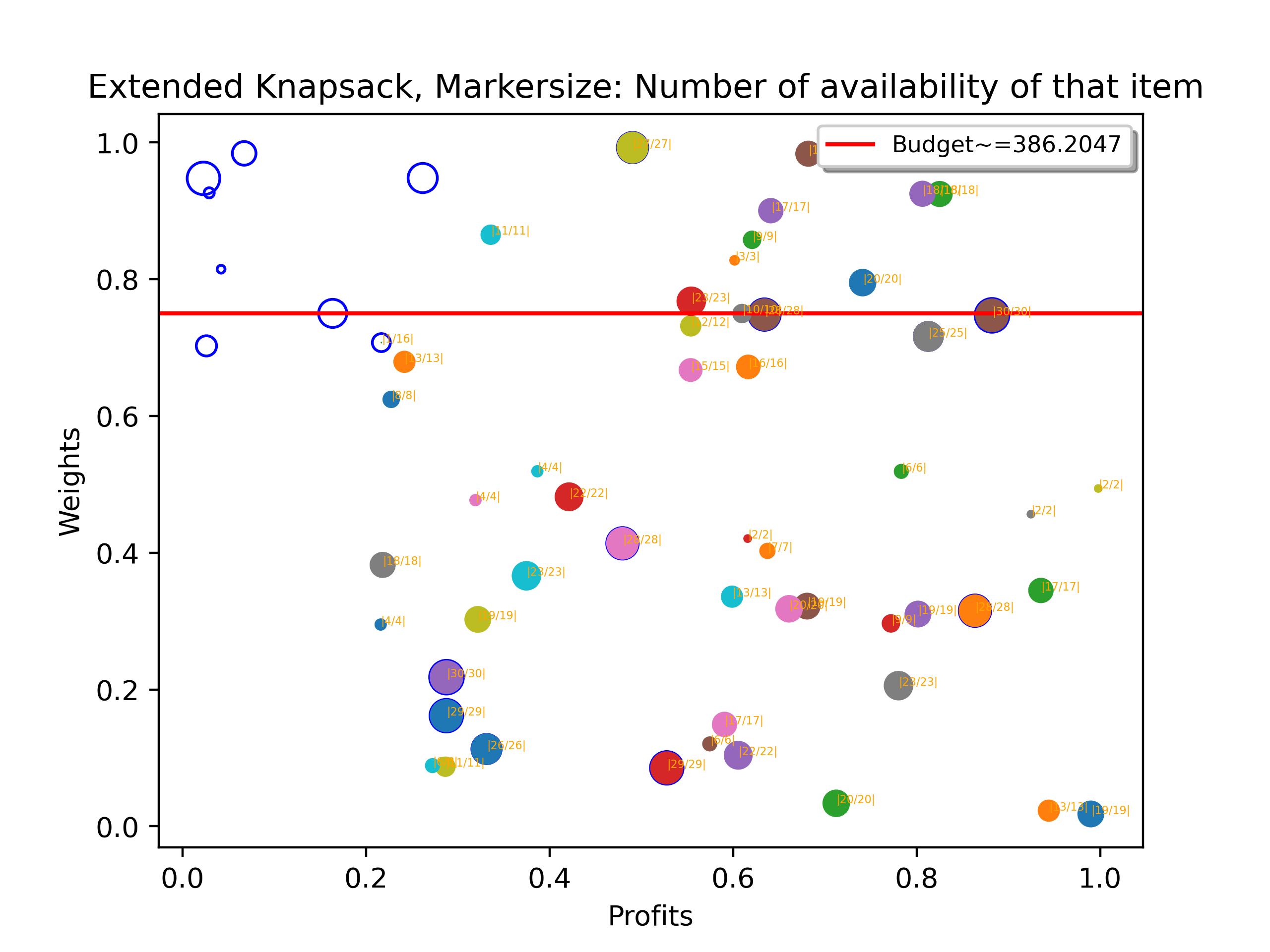
Here is 3 instances of the solutions visualized using matplotlib.pyplot.
-
Horizontal Line/Axis:
- The horizontal red bar is representing the budget, the y offset is budget/(total weights of all the items)
- Circles are plotted on the coordinate system where y: weights, x: profits.
-
Circles:
- The items in the knapsack.
- The color is random, it looks like skittle, but if a circle is fulled by color, then it represents that that item is included into the optimial solution.
- The size of the circle represents the number of items available with that exact weights and profits in the knapsack.
- The coordinate of the circles corresponds to the weight and profits of the item.
- The label on the circle is in the format of "\|\d+/\d+\|", where the first number represents the number of that items that is included into the final optimal solution, the second number represents the availability of that items in the knapsack.


