Intro

We discuss the conjugate gradient algorithms in details and then we move on and show its application in deblurring images that is blurred by box blur kernel with odd sizes.

Here is a list of things that are going to be discussed on this webpage:

1. Conjugate Gradient Algorithm
   • Conjugate Direction and Conjugation Process
   • Proof
   • The algorithmic implementation
   • Augmentations and adaptations
2. Box Blur
   • Kernel convolution on image is matrix vector multiplications
   • Box Blur's matrix representation is a symmetric matrix
3. Applying the conjugate gradient algorithm for deblurring imaged blurred by box blur

Here is what is needed from the readers:

• Knows non-trivial amount of multi-variable calculus and linear algebra.
• Knows non-trivial amount of python programming.
• Has a background on Scientific Computing.

Here is what recommended to know in advanced so that reading can be sped up for the readers

• Properties of the Hermitian Matrices
• The Gram Schmidt Process
• Image Processing
• Positive Definite Matrix
• Graphs and Adjacency Matrix
• Basics about iteratives solvers for linear systems
• Gradient Descend: Steepest Descend

Why all the "Prerequisite"?

It's not that I want to limit the readers for this webpage, it's just that if I were to explain everything from the ground up, this website will be 200 pages long.

Why are all these math necessary?

A lot of programmer won't care about this, but they will be making a big mistake by not knowing it from a deeper level, it will inhibit their creativity when it comes to problem solving, limit their ability to find noval applications for the algorithms and then when the algorithms failed to do what they expected, blaming the algorithm instead of knowing exactly why and suggest alternatives.
Personally, I love the math and it's the math that make the Conjugate Gradient Algorithm special. It has a very interesting flavor to it.

Jupyter Notebook

Some of the experimentation with my homebrewed conjugate gradient can be found here in a jupyter notebook.

Conjugate Gradient Method

Conjugate gradient is a class of optimizers for linear system. Some of other solvers of the same types includes: Bi-Conjugate Gradient, Bi-Conjugate Gradient Stabalized, and Generalized Minimial Residual Method, GMRes.

These class of algorithm is iterative, meaning that it approximates the solution to the linear system $Ax = b$ better and better. They also comes with the advantage of not requiring to know what numbers are in the matrix $A$, unlike direct method such as Gaussian Eliminations, Cholesky or LU Decomposition. It can figure out the solution purey by interacting with the linear operator $A$.

Their major applications are for solving PDEs, where differential operators such as the Laplacian are used and they needs to be inverted.

Claim 1

The solution to: $$ \arg\min_{x}\left\lbrace \frac{1}{2}x^TAx - b^T x + c \right\rbrace $$ Is the solution to $Ax = b$ if $A \in \mathbb{R}^{n\times n}$ is Symmetric Positive Definite (SPD)

Proof

The problem has a minima becase $A$ is positive definite, meaning that $x^TAx$ is always going to be larger than zero, therefore it's bounded from below and has a minima.

The minima can be computed via:

$$ \begin{aligned} f(x) &=\frac{1}{2}x^TAx - b^T x + c \\ \nabla_x[f(x)] &= \frac{1}{2}(A^T + A)x - b \\ \underset{[1]}{\implies} \nabla_x[f(x)] &= Ax - b \\ \text{Let: }\quad \nabla_x[f(x)] &= 0 \\ \implies Ax & = b \end{aligned} \tag{1} $$

[1]: $A + A^T$ is $2A$ because $A$ is symmetric

Claim 1 is proven $\blacksquare$

Inspirations for Conjugate Gradient

Steepest descend method doesn't work well when the matrix is not well conditioned. It will oscilates along the direction and slowly zig zag to the minimal, turning exactly 90 degress each time. We want a smart way of choosing the direction to descend to such that the energy normal always decrease. (The energy norm: $\Vert x\Vert_A^2 = x^TAx$)

Conjugate Vectors

Vector $u, v$ are conjugate if $u^TAv = 0$ for some $A$ that is PD (Positive Definite)

Let $x^{(i)}$ be the solution approximated at $i$ th step of the algorithm, let $d^{(i)}$ be the direction of descend chosen at $i$ th iterations of the algorithm, then, we want the algorithm to statisfies the following:

$$ x^{(k + 1)} = x^{(k)} + \alpha_{k} d^{(k)} \tag{2} $$ $$ d^{(k + 1)} \perp \left\langle d^{(1)}, d^{(2)}, \cdots, d^{(k)} \right\rangle_A \tag{3} $$

Where, the direction from the $k + 1$ th iteration is conjugate to all previous search direction and $\alpha$ is a step size that is left to be determined.

Before we start, let's define a list of quantities that we are going to use:

Defined Quantities

1. $Ax_+ = b$
2. $e^{(i)} = x^{(i)} - x_+$
3. $r^{(i)} = b - Ax^{(i)}$
4. $r^{(i)} = -Ae^{(i)} = -A(x^{(i)} - x_+) = -Ax^{(i)} + b$
5. $r^{(i)} = -\nabla_x[f](x^{(i)})$

Claim 2

By representing the error vector as a linear combinations of the conjugate vectors, we an show that the algorithm termintes after at most n steps of literations, if we walk along the direction $d^{(k)}$ such that it minimizes the objective function $f(x)$. $$ \begin{aligned} e^{(0)} &= \sum_{j = 0}^{n - 1}\delta_jd^{(j)} \end{aligned} \tag{4} \implies e^{(n)} = \mathbf{0} $$

Claim 3

The step size into the conjugate direction: $\alpha_k$ is the same as the weight given to representing the error vector as linear combinations of the conjugate directions, and it also gives the steepest descend along the conjugate direction for the objective function. $$ \delta_k = -\alpha_k \tag{5} $$

Consider Claim 2

$$ \begin{aligned} e^{(0)} &= \sum_{j = 0}^{n - 1}\delta_jd^{(j)} \\ Ae^{(0)} &= \sum_{j = 0}^{n - 1} \delta_j Ad^{(j)} \\ d^{(k)}Ae^{(0)} &= \underbrace{\sum_{j = 0}^{n - 1} \delta_j d^{(k)T}Ad^{(j)}}_{\delta_kd^{(k)}Ad^{(k)}} \\ \delta_k &= \frac{d^{(k)T}Ae^{(0)}} { d^{(k)T}Ad^{(k)} } \\ \underset{ [1] } {\implies} \delta_k &= \frac{ d^{(k)T}A(e^{(0)} + \sum_{j = 0}^{k-1} \alpha_jd^{(j)}) } { d^{(k)T}Ad^{(k)} } \\ \underset{[2]}{ \implies } \delta_k &= \frac{ d^{(k)T}Ae^{(k)} }{ d^{(k)T}Ad^{(k)} } \\ \delta_k &= \frac{-d^{(k)T}r^{(k)}}{\Vert d^{(k)}\Vert_A^2} \end{aligned} \tag{6} $$

[1]: At this point, we just added $\sum_{j = 0}^{k - 1}\alpha_jd^{j}$, but because all the $d^{(i)} \;\forall\; 0 \le i \le k - 1$ are $A$ orthogonal to $d^{(k)}$, so expanding it out will just give us zero.
[2]: Because $e^{(k)} = x^{(k)} - x^{+} = x^{(0)} + \sum_{j = 0}^{k - 1}\alpha_kd^{(k)} - x^{+} = e^{(0)} + \sum_{j = 0}^{k - 1}\alpha_kd^{(k)}$. Recalled section Defined Quantities.

Claim 3 Proof

Optimizing the function along the conjugate direction requires considering the optimality conditions forest, by taking the derivative wrt $\alpha_k$ and then set it to zero:

$$ \begin{aligned} \partial_\alpha [f(x^{(k + 1)})] &= \partial_\alpha[f(x^{(k)} + \alpha d^{(k)})] \\ &= \nabla_x[f(x^{(k + 1)})]^Td^{(k)} \\ \text{set:}\quad \partial_\alpha [f(x^{(k + 1)})] &= 0 \\ \underset{[1]}{\implies} r^{(k + 1)T}d^{(k)} &= 0 \\ \implies Ae^{(k + 1)T}d^{(k)} &= 0 \end{aligned} \tag{7} $$

[1]: Recall that $r^{(k)} = b - Ax^{(k)}$ and $\nabla_x[f(x)] = Ax - b$ from Defined Quantities.

However, the optimality conditions doesn't seem to involve the qautntity $\alpha$ explictly, therefore we need to find it by expanding on $e^{(k + 1)}$, so then we have:

$$ \begin{aligned} r^{(k + 1)T}d^{(k)} &= 0 \\ [b - Ax^{(k + 1)}]^Td^{(k)} &= 0 \\ [b - A(x^{(k)} + \alpha_k d^{(k)})]^Td^{(k)} &= 0 \\ [b - Ax^{(k)} - \alpha_k A d^{(k)}]^Td^{(k)} &= 0 \\ [r^{(k)} - \alpha_k Ad^{(k)}]^Td^{(k)} &= 0 \\ \alpha_k &= \frac{r^{(k)T}d^{(k)}}{d^{(k)T}Ad^{(k)}} \\ \alpha_k &= \frac{r^{(k)T}d^{(k)}} { \Vert d^{(k)}\Vert_A^2 } \end{aligned}\tag{8} $$

Compare $\alpha_k$ with $\delta_k$ from (8) and (7) and observe that claim 3 has been proven. $\blacksquare$

Using the fact from claim 3, and then the definition of $e^{(0)}$, observe that if conjugate gradient is tshe search direction and we use the $\alpha_k$ found in the proof, then claim 2 is proved as well. $\blacksquare$

Morals of the story so far

As we can see, there is indeed a way of choosing the directions of descend such that the convergence after $n$ interations is promised, and we can also observe that, the error vector, when measured using energy norm, is always decreasing too. $\Vert e^{(k + 1)}\Vert \le \Vert e^{(k)}\Vert_A$.

Intuitions

As explained in different literatures, there are a lot of different interpretations in choosing conjugate direction and how it exactly decreases the objective function in such an optimal way.

Most literatures explain it that, the algorithm will choose the search direction such that the energy norm with matrix $A$ is decreased as much as possible.

Some other suggests the geometric interpretation of the fact that conjugate vectors are orthogonal after being transformed with matrix $A^{-1}$, and it's up to the reader to know that $A^{-1}$ exists when $A$ is symmetric and positive definite.

Well, my interpretations is based on eigenvectors. If you make $d^{(0)}$ to be the eigenvector of $A$, then the algorithm will find the solution right away because the eigenvector of the Hermitian Matrix has the geometric interpretations that they are the principal axis of the transformation. (Or some algebra can also be a convincing argument)
In addition, using the fact that eigenvectors of matrix $A$ are orthogonal, then eigenvectors they are conjugate of each other. And, if the vector $u, v$ when represented under the eigenspace are orthogonal, it's not hard to see that they will also be orthogonal. Now recall that Eigenvectors are also the principal axises for the transformations of the Hermitian matrix. Think about it in your head and you will know why everything makes sense. That is my interpretation.

There is still a Big Problem

How do we find Conjugate Vectors as search direction for the algorithm?

Gram Schimdt Conjutation

It's the same idea as the Gram Schimdt orthogonalization process, but this time we wish to produce conjugate vectors instead of orthogonal vectors.

• GS Conjugation: Orthogonal Vectors $\rightarrow$ Conjugate Vectors
• GS Orthogonalization: Any Linearly Independent vectors $\rightarrow$ Orthogonal Vectors

Given a set of orthogonal vectors $\{u_i\}_{i = 1}^n$ that spans the whole $\mathbb{R}^{n}$ (Standard Basis vectors are an ok choice here), where, the matrix $A$ is $n\times n$.
To construct a set of vectors that are $A$ orthogonal, we would need to subract from the vector $u_i$ with components span by the vectors $d^{(i< k)}$. Mathematically: $$ \begin{aligned} d^{(k)} &= u_{k} + \sum_{i = 1}^{k - 1} \beta_{k, i} d^{(i)} \end{aligned} \tag{9} $$

Looking for $\beta_{k, i}$

Exercise for the Readers

Reformulate the GS Conjugation without the orthogonality assumption on $u_k$. I will be too easy on the readers if it's just me who is doing the math. Regardless of who you are, I encourage you to think about it, because you are reading it, you should think about it even if you are a recruiter who stumbled upon my websites.

The Magical Ingredient: $r^{(k)}$

Using the residual vector the guide the generative process of the conjugate directions will tremendously reduce the complexity of the GS conjugation, because it won't need all previous $d^{(i < k - 1)}$ vectors anymore.

Claim 4

The residual direction at the $j$ of the iteration is orthogonal to all previous conjugate direction, assuming conjugate directions for the steepest gradient descend, mathematically: $$r^{(j)T}d^{(i)} = 0 \quad \forall i < j$$

Claim 4 Proof

Recalled from Defined Quantities, let $i < j$ and Consider

Claim 4 is proven $\blacksquare$

Claim 5

In addition to $r^{(k)}$ being orthogonal to all previous conjugate vectors, it's also authogonal to all previous $u_i$ that assists with the generative process of the conjugate vectors. $$r^{(i)}\perp u_{j} \quad \forall i < j$$

Claim 5 Proof

Choose $j > i$ then consider:

Observe that, choosing $i = j$, we have $r^{(i)T}d^{(i)} = r^{(i)T}u_i$

Claim 5 is proven $\blacksquare$

Claim 6

We are getting close to the essence of the conjugate gradient algorithm.

Using the residual vector during the iterations will simplify the GS Conjugation process significantly. basically let $u_i = r^{(i)}$.

Claim 6 Justification

Congrat you made all the way to here, the next few steps is basically using the residual vectors during the iterations as the set of $\{u_i\}_{i = 1}^n$ for assisting the generation of the conjugate search directions.

From the Gram Schimdt conjugation process we have: $$ \beta_{k, m} = - \frac { d^{(m)T}Au_{k} } { \Vert d^{(m)}\Vert_A^2 } $$ Let $u_k = r^{(k)}$ then $\beta_{k, m} = \frac{d^{(m)T}Ar^{(k)}}{\Vert d^{(m)}\Vert_A^2}$ and we need to find $r^{(k)T}Ad^{(m)}$.

Consider the residual at the $j + 1$ iteration of the algorithm then: $$ \begin{aligned} r^{(j + 1)} &= -Ae^{(j + 1)} \\ &= -A(e^{(j)} + \alpha_{j} d^{(j)}) \\ &= r^{(j)} - \alpha_{j} Ad^{(j)} \\ r^{(i)T}r^{(j + 1)} &= r^{(i)T}r^{(j)} - \alpha_{j} r^{(i)T}Ad^{(j)} \\ \alpha_{j}r^{(i)T}Ad^{(j)} &= r^{(i)T}r^{(j)} - r^{(i)}r^{(j + 1)} \end{aligned} \tag{14} $$

Now, there are several cases of values for $\alpha_i$, and it depends on the value of $i, j$.

• Consider $i < j$, from claim 5, replacing $u_j$ with $r^{(j)}$, when $i < j$, the right handside is always zero, which implies that $\beta_{i, j} = 0$.
• When $i = j$ it's $\Vert r^{(i)}\Vert_2^2$, however we don't need this for the conjutation, it's not in the summation.
• Consider $i = j + 1$, then

The only quantity left is when $i = j + 1$, and therefore, we only need to keep the residual vector from the preious iterations and the conjugate direction to figure out the next conjugate search direction. At this point, claim 6 has been justified. $\blacksquare$

The Conjugate Gradient Algorithm

Now, we have all the components for the Conjugate Gradient Algorithm. Let's take a look at the quantities that need to be updated and maintained throughout the algorithm

• $\alpha_k$, the step size into the conjugate direction.
• $\beta_{k + 1, k}$, the weighting for the next conjugate direction.
• $r^{(k)}$, $d^{(k)}$, $x^{(k)}$, the usual deal.

Let's consider $\beta_{i + 1, i}$, and recall that from claim 3, we have $\alpha_k = \frac{r^{(k)T}d^{(k)}}{\Vert d^{(k)}\Vert_A^2}$

Recall from the proof of claim 5, with the observation $r^{(i)T}d^{(i)} = r^{(i)}u_i$, and we know that $u_i = r^{(i)}$, then we have: $$ \begin{aligned} \alpha_k &= \frac{r^{(k)T}r^{(k)}}{\Vert d^{(k)}\Vert_A^2} \\ \implies \beta_{j + 1, j} &= \frac{\Vert r^{(j + 1)}\Vert_2^2}{\Vert r^{(j)} \Vert_2^2} \end{aligned} $$

And here is the final updating sequence for each of the variable, for notation convenience, $\beta_{i + 1, i}$ is $\beta_{i + 1}$, and then we have: $$ \begin{aligned} d^{(0)} &= b - Ax^{(0)} \\ \alpha_{i} &= \frac{\Vert r^{(i)}\Vert_2^2} {\Vert d^{(i)}\Vert_A^2} \\ x^{(i + 1)} &= x^{(i)} + \alpha_i d^{(i)} \\ r^{(i + 1)} &= r^{(i)} - \alpha_iAd^{(i)} = b - Ax^{(i + 1)} \\ \beta_{i + 1} &= \frac{\Vert r^{(j + 1)}\Vert_2^2}{\Vert r^{(i)}\Vert_2^2} \\ d^{(i + 1)} &= r^{(i + 1)} + \beta_{i + 1}d^{(i)} \end{aligned} $$

CG implemented Python

                
def AbstractCGGenerate(A:callable, b, x0, maxitr:int=100):
    """
        A generator for the Conjugate Gradient method, so whoever uses it
        has the pleasure to collect all the quantities at runtime.
    :param A:
    :param b:
    :param x0:
    :return:
        itr, r, x
    """
    x = x0
    d = r = b - A(x)
    Itr = 0
    while Itr < maxitr:
        alpha = np.sum(r * r) / np.sum(d * A(d))
        if alpha < 0:
            warnings.warn(f"CG negative energy norm! Matrix Not symmetric and SPD! Convergence might fail.")
        x += alpha * d
        # rnew = r - alpha * A(d)
        rnew = b - A(x)
        beta = np.sum(rnew * rnew) / np.sum(r * r)
        d = rnew + beta * d
        r = rnew
        Itr += 1
        yield Itr, r, x
                
            

A list of Things for the Algorithm

• It's a generic subroutine.
• For better numerical precision, we implemented $b - Ax^{(i + 1)}$ for getting the residual
• The algorithm almost never converge complete after $n$ iterations because of numerical instability
• This algorithm treat $A$ as a blackbox, and all vectors can be left as tensor, representing images, or whatever it's under the concern for the linear operator, but it has to be a numpy arrray type
• The positive definite precondition of the algorithm puts a warning for the user instead of asserting it.
• This algorithm doesn't support the use of preconditioners because I haven't talk about thta part yet.

Exercise for the Readers

I don't care who you are, but doing this will enhance your understanding of what we just discussed.

1. Implement this in C/C++.
2. Extra points if it's implemented on GPU. Extra Extra points if it supports preconditioners.
3. Extra Extra Extra points if you got both.
4. Go do your doctoral thesis if you can improve the numerical stability for badly conditioned $A$.(You should not be goofying around on my website and reading this if that is the case).

THE END of Vanilla Conjugate Gradient

Adaptations and Augmentaions for Conjugate Gradient

This section is concerned about applying the algorithm to different situations, and potential interesting behaviors when it's not used properly. Keep in mind that, if an approximation matrix $M$ is found for $A$, then preconditioners can be applied to improve the convergence of the algorithm, but that is skipped here.

Symmmetric Positive Semi-Definite Matrices

Suppose that matrix $A$ is positive semi-definite, meaning that $\exists x: x^TAx = 0$, then according to claim 1, the problem has infinitely many solutions, and it's up to the initial guess to say which one the algorithm will land us on.
One can find the use of adding some extra terms for the objective function useful, potentially limiting the number of solutions. But such an approach will involve changing the algorithm a bit to support the regularizations.

Symmetric Matrices

If given matrix that is only symmetric, then it's possible that it's positive semi-definite, negative semi-definite, or definite. In such cases, CG can't be diretly applied.

Assuming that $A$ is Negative Definite, or Semi-Definite

Then $-A$ is positive definite or semi-definite. Solve $-Ax = -b$ instead, or make it into gradient ascend instead of descend.

Assuming $A$ is Neither

Consider

$A$ is not Symmetric

Then $A^TA$ is symmetric, solve $A^TA = A^Tb$ instead, at the cost of poorer conditioning and there is no way of treating the problem as a blackbox anymore. Or, consider using GMRes algorithm, which is applicable for all types of matrices and it's able to treat then as a blackbox.

Box Blurring

Let the kernel size be $m\times n$, and let the image be represented by a tensor $M$, so then it's $\text{Height}\times \text{Width} \times 3$, then the output image, called it $\widetilde{M}$, is going to be: $$ \begin{aligned} \widetilde{M}[i, j, k] = \sum_{\alpha = i - \frac{m}{2}}^{i + \frac{m}{2}} \sum_{\beta = j - \frac{n}{2}}^{j - \frac{n}{2}} \frac{1}{mn} M \left[ \alpha \% \text{Height}, \beta \% \text{Width}, k \right] \end{aligned} $$ Where $\%$ is the modulo operator. Notice that this is a linear transform because the new pixel is expressed as the weighted sum of it's neigbouring pixels. Observe that this is only for periodic boundary conditions and for our purposes we will only consider blurring algorithm that doesn't change the shape after transformation, which means limiting the type of boundary conditions for the blurring algorithm.

Claim 7

For the box blur kernel, when it's odd size and it's a box, it's can be represented by a symmetric matrix. An odd size kernel is $$\text{Kernel}\in \mathbb{R}^{(2m + 1)\times (2m + 1)}\quad \forall m \in \mathbb{Z}_{\ge 0} \wedge m \le \left\lfloor\frac{\min(\text{Height}, \text{Width})}{2}\right\rfloor$$
To rephrase the above statement and be more specified, we want to show that:
Let $A$ reprents the operators for box blurring, and it's a $(m\times n\times 3) \times (m\times n\times 3)$ matrix, for the image $M$. Let's also define the vectorized image to be all the rows from the imagee stacked into a vector $x$, mathematically: $$ \text{vec}(M) = \begin{bmatrix} M[1, :, 1] \\ M[2, :, 1] \\ \vdots \\ M[\text{Height}, :1] \\ M[1, :, 2] \\ M[2, :, 2] \\ \vdots \\ M[\text{Height}, :2] \\ M[1, :, 3] \\ M[2, :, 3] \\ \vdots \\ M[\text{Height}, :3] \end{bmatrix} $$ Where $\text{vec}$ denotes the bidirectional vectorization procedures given any tensor, so then we can say that: $$ \exist A \in \mathbb{R}^{(\text{Height} \times \text{Width}\times 3)\times(\text{Height} \times \text{Width}\times 3)}: \text{vec}(\widetilde{M}) = A (\text{vec}(M)) \wedge A^T = A $$

Note

Any order of vectorization on the fiber of tensor $M$ going to be the same, but each of them will have a different $A$, but all symmetric.

Claim 7 Proof Strategy

To prove that, we will need to show that the $k$ th column and rows of the matrix $A$ are the same. Now, listen carefully, because I will be clarifying what the rows and the clumn of the matrix is doing to every pixel in the image.

• The $i$ row of the matrix tells us how each pixel at position $\left\lfloor \frac{i}{\text{Width}}\right\rfloor + i\% N$ for all 3 layers are affected by values of its neighbours.
• The $i$ column of the matrix $A$ tells us how each pixel at position $\left\lfloor \frac{i}{\text{Width}}\right\rfloor + i\% N$ is contributing to the sum of its neighbours.
• We want to show thta these 2 vectors are the same

Proof

1. From each pixel, draw an weighed outgoing edge to its neigbours that is going to be summed up by the box kernel, and the weight is the $1/(2m + 1)^2$
2. For each pixel, draw an weighted incoming edge from its neigbours that is included by the box kernel if the piexel is going to be summed up by it's neighbours.
3. Construct such a weighted digraph on all pixels for all 3 layers.
4. All edges on the graph is bidirectional and has the same weight for both direction by definition above and how box blur works
5. The Adjacency matrix of this graph is the matrix $A$.
6. Because of reason (5.), (4.), the matrix symmetric.

About this Proof

I was talking to my friend, go by the name Nost on discord about this. I was inspired by his graphical intereptation by the convolutional procedures, and then came out with this proof 40 mins after finishing reading about the Arnoldi Iterations.

Exercise for the Readers

Listen again, I don't care who you are, but if you are reading this you need to think. Here is the question I have for you:

• Using the above $\text{vec}$ we defined, come up with an compact expression for the matrix $A$, for periodic boundary conditions.

Hint: Use Kron Product and some matrix that shifts the rows. It should have a really good structure to it.

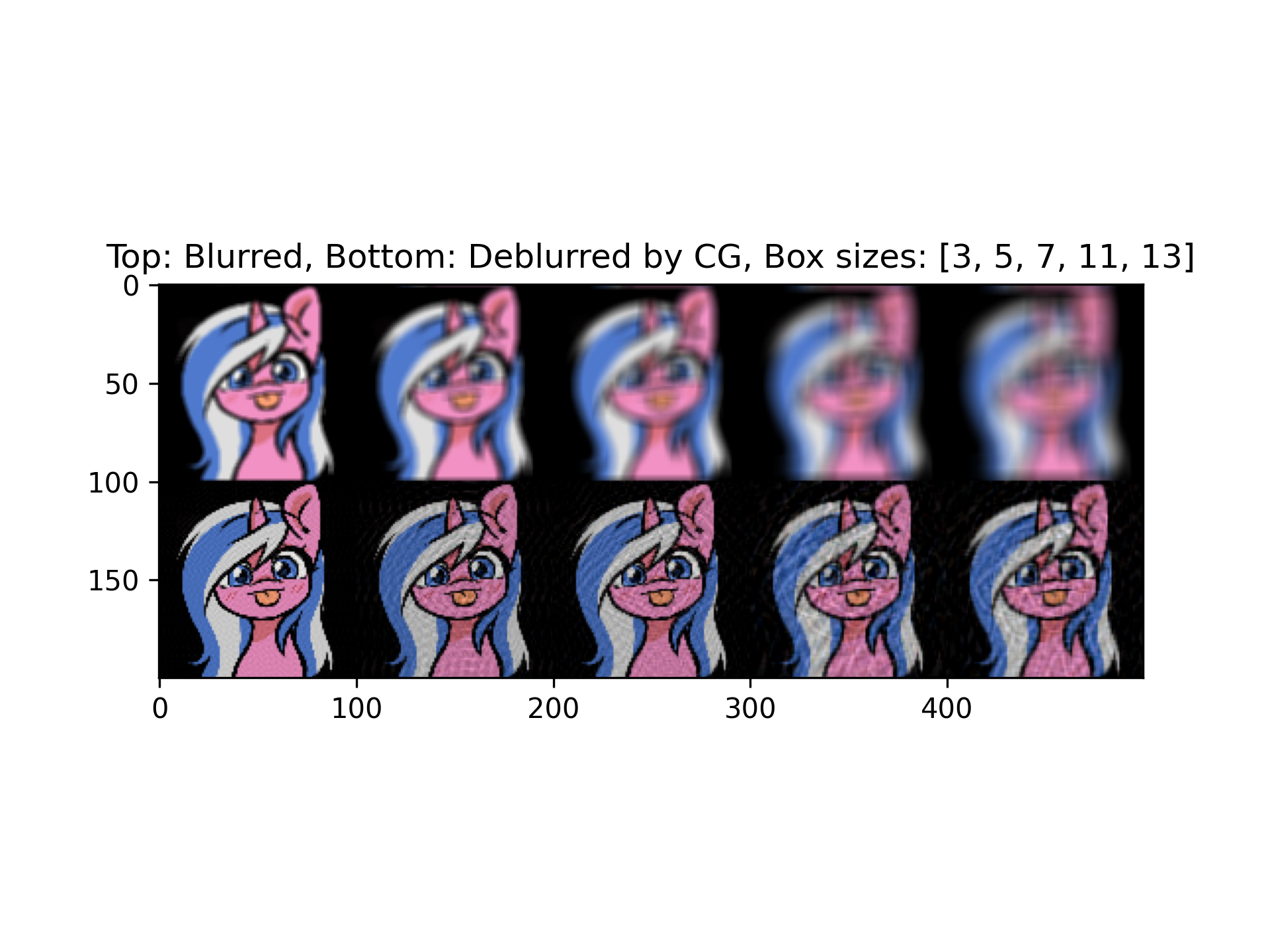
Some Results when Applied to Deblurring

Here is a deblurring carried out on my Unicorn OC:

Here is a deblurring carried out on the character Snow Drop, also my friend's choice:

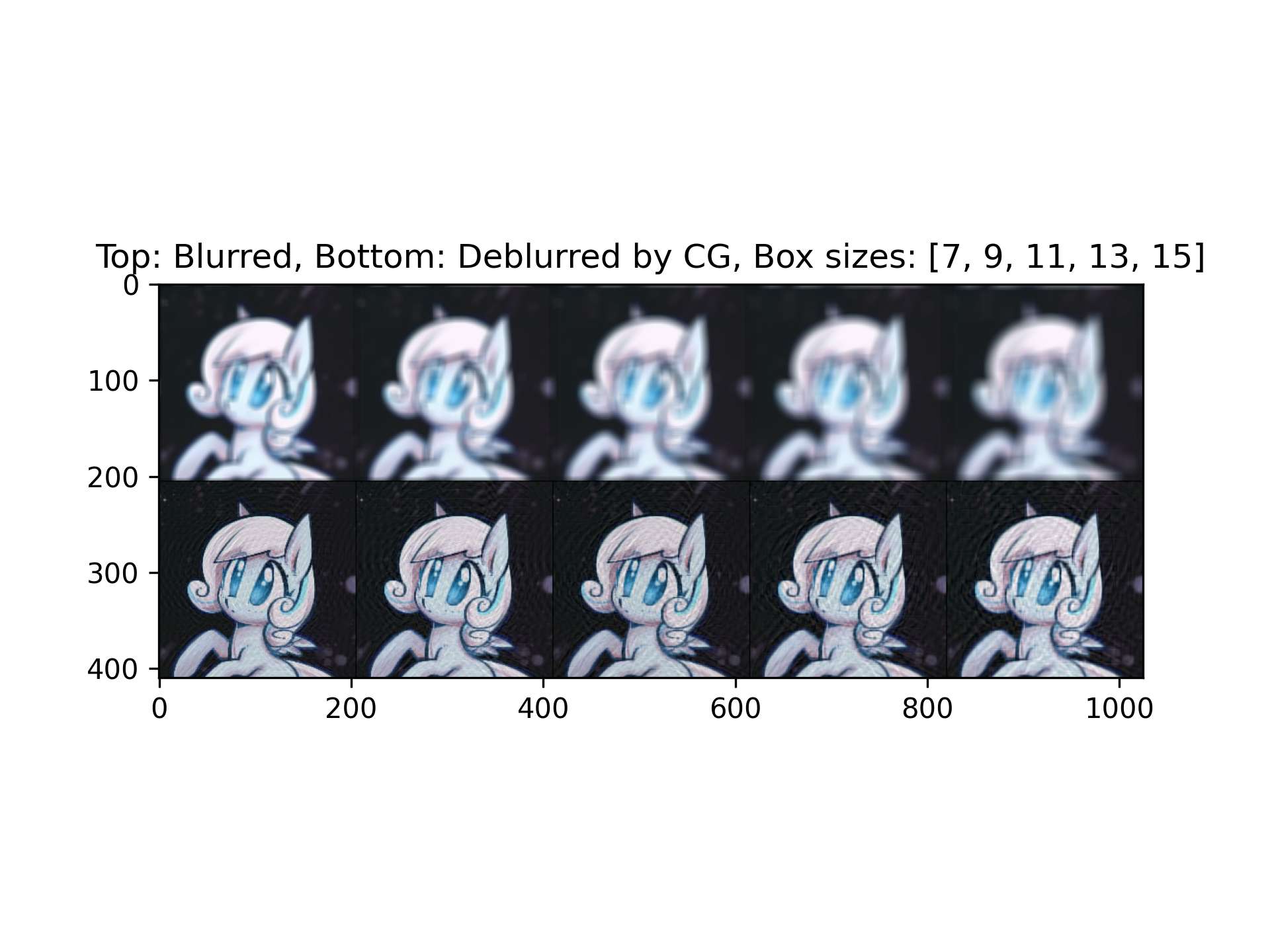
Python implementation here.

For more experimentation on more aggressive blurring that involves multiple successive kernel passes, go back to the intro to look for the Jupyter Notebook link.

Exercise for the Readers

Go read my Jupyter notebook and and answer:

• What type of symmetric matrix is the box blurring operator with square odd sizes?

Epilogue

Firstly, to make sure you actually read and understand it, discuss the exercise with me, my email is on the top right corner of the main page.

Secondly, I didn't talk about preconditioners, and judging by how much efforts are involved to put together this website, I might never talk about it in here. Therefore...

Excercise for the Readers

Implemenet the Conjugate Gradient Method with Preconditioning for the matrix, and apply it to box deblurring, compare the decay of the Energy Norm of the error vector $e^{(k)}$ to show that your shoice of preconditioners worked well.

References